When we would like to create a decision tree we can choose from many possibilities, but formatting the tree is not always that easy. I will show a way to create, format a tree and list the rules of the inner nodes. Being able to read this rules can be very useful by an analysis. I will use the partykit package. Besides that we will need the data.table package by listing the rules of the inner nodes and optionally the xlsx package if we want to save these rules in an xls.
> library(xlsx)
> library(partykit)
> library(data.table)
I am using randomly generated data. In this example I am selling jeans and I am curius about on what depends the period of selling different type of jeans. I have data about 10000 sales including the fit (straight, bootcut or skinny), length (short or normal), color (blue, black, red or yellow) and price (10-124 $) of the jeans and the number of days of the sale of it (0-3 days, 4-14 days or more).
> head(data)
  Days      Fit Price $ Color Length
2  0-3 Straight      81   Red Normal
3  0-3 Straight      61   Red  Short
1 4-14  Bootcut      87   Red Normal
4 4-14  Bootcut      47   Red Normal
5 4-14   Skinny      82   Red Normal
6 4-14 Straight      88 Black Normal
> nrow(data)
[1] 10000
In order to estimate the accuracy of our model, I will split my data to a training and a test dataset.
> set.seed(9898)
> testind<-sample(c(1:nrow(data)), nrow(data)*0.2)
> test<-data[testind,]
> train<-data[-testind,]
The tree and the prediction:
> tree<-ctree(Days~., data=train, mincriterion = 0.99)
>
> test$predict<-predict(tree, newdata = test, type = "response")
By fitting the model we could control the testtype, the size of the tree, the splitting criterias etc. as well with a list of parameters in the control = ctree_control() argument. Now I only set the mincriterion, it is the value of 1-p, a split will be implemented only by exceeding this value, which is strenger by the default.
The accuracy of the modell is 0.622, which is quite good. Without the model only with guessing our accuracy would be about 0.33 (since the explained variable has 3 values), so 0.631 is a great improvement.
> test$match<-0
> test$match[which(test$predict==test$Days)]<-1
> accuracy<-sum(test$match)/nrow(test)
> accuracy
[1] 0.631
Now I am visualizing my tree. First I define the colors. The columncol means the colors of the columns in the terminal nodes, the labelcol the background colors of the labels in the inner nodes and the indexcol the bacground colors of the indexes.
> columncol<-hcl(c(270, 260, 250), 200, 30, 0.6)
> labelcol<-hcl(200, 200, 50, 0.2)
> indexcol<-hcl(150, 200, 50, 0.4)
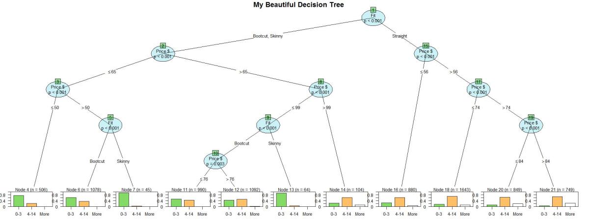
The imaged will be saved immediately as Tree.jpg in the working directory.
> jpeg("Tree.jpg", width=2000, height=750)
> plot.new()
> plot(tree, type = c("simple"), gp = gpar(fontsize = 15),
+      drop_terminal = TRUE, tnex=1,
+      inner_panel = node_inner(tree, abbreviate = TRUE,
+                               fill = c(labelcol, indexcol), pval = TRUE, id = TRUE),
+      terminal_panel=node_barplot(tree, col = "black", fill = columncol[c(1,2,4)], beside = TRUE,
+                                  ymax = 1, ylines = TRUE, widths = 1, gap = 0.1,
+                                  reverse = FALSE, id = TRUE))
> title(main="My Beautiful Decision Tree", cex.main=3, line=1)
> dev.off()
And here is the tree:

Maybe it would be important to see according to what kind of rules was the data partitioned. Now I list these rules produced for each class. With this script we will get the results in formatted, and it will be saved as an xls file.
First I save in the terminals the predictions and the rules how have we got them.
> terminals <- data.frame(response = predict(tree, type = "response"))
> terminals$prob <- predict(tree, type = "prob")
>
> rules<-partykit:::.list.rules.party(tree)
> terminals$rule <- rules[as.character(predict(tree, type = "node"))]
Then I format and aggregate the values and the variablenames and I save it as Rules.xls.
> value<-cbind(terminals$rule, terminals[,which(grepl("prob", colnames(terminals)))])
> colnames(value)[1]<-"rules"
> DF<-data.table(value)
> terminals<-as.data.frame(DF[,sapply(.SD, function(x) list(max=max(x))),by=list(rules)])
> terminalsname<-cbind(names(rules), rules)
> terminals<-merge(terminals, terminalsname, by=c("rules"))
> names<-colnames(terminals)[which(grepl(".max", colnames(terminals)))]
> names<-unlist(strsplit(names, "[.]"))[-which(unlist(strsplit(names, "[.]"))=="max")]
> colnames(terminals)[which(grepl(".max", colnames(terminals)))]<-names
> colnames(terminals)[which(colnames(terminals)=="V1")]<-"Terminal_Node"
> colnames(terminals)[which(colnames(terminals)=="rules")]<-"Rule"
> terminals<-terminals[,c(5,1,2,3,4)]
> terminals$Rule[which(grepl("\"NA\"", terminals$Rule))]<-gsub("\"NA\"", "", terminals$Rule[which(grepl("\"NA\"", terminals$Rule))])
> terminals$Terminal_Node<-as.numeric(as.character(terminals$Terminal_Node))
> terminals<-terminals[order(terminals$Terminal_Node),]
> write.xlsx(terminals, "Rules.xls", row.names=FALSE)
So here are the decision rules.
You can learn more about decision trees here or here.
| Terminal_Node | Rule | 0-3 | 4-14 | More |
| 4 | Fit %in% c(“Bootcut”, “Skinny”) & Price $ <= 65 & Price $ <= 50 | 0.77 | 0.23 | 0.00 |
| 6 | Fit %in% c(“Bootcut”, “Skinny”) & Price $ <= 65 & Price $ > 50 & Fit %in% c(“Bootcut”, ) | 0.62 | 0.37 | 0.00 |
| 7 | Fit %in% c(“Bootcut”, “Skinny”) & Price $ <= 65 & Price $ > 50 & Fit %in% c(“Skinny”, ) | 0.96 | 0.04 | 0 |
| 11 | Fit %in% c(“Bootcut”, “Skinny”) & Price $ > 65 & Price $ <= 99 & Fit %in% c(“Bootcut”, ) & Price $ <= 76 | 0.54 | 0.45 | 0.01 |
| 12 | Fit %in% c(“Bootcut”, “Skinny”) & Price $ > 65 & Price $ <= 99 & Fit %in% c(“Bootcut”, ) & Price $ > 76 | 0.45 | 0.52 | 0.03 |
| 13 | Fit %in% c(“Bootcut”, “Skinny”) & Price $ > 65 & Price $ <= 99 & Fit %in% c(“Skinny”, ) | 0.92 | 0.08 | 0 |
| 14 | Fit %in% c(“Bootcut”, “Skinny”) & Price $ > 65 & Price $ > 99 | 0.25 | 0.63 | 0.13 |
| 16 | Fit %in% c(“Straight”) & Price $ <= 56 | 0.27 | 0.64 | 0.09 |
| 18 | Fit %in% c(“Straight”) & Price $ > 56 & Price $ <= 74 | 0.17 | 0.70 | 0.13 |
| 20 | Fit %in% c(“Straight”) & Price $ > 56 & Price $ > 74 & Price $ <= 84 | 0.13 | 0.66 | 0.21 |
| 21 | Fit %in% c(“Straight”) & Price $ > 56 & Price $ > 74 & Price $ > 84 | 0.07 | 0.68 | 0.25 |
