
There are different selection methods for multiple linear regression to test the predicting variables, in order to increase the efficiency of our analysis. Variable selection is a contested topic but in some cases it can be useful. I am going to take a review of four common methods (enter, forward selection, backward elimination, stepwise selection) and check the differences in the results with bootstrapping (number of incidences: 100).
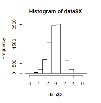
In my example I use random data following normal distribution with some correlation between the variables. X is the dependent variable and A, B, C, D and E are the independents.
> head(data)
           X          A          B          C          D            E
1  0.5029670 -0.5410024  1.1435710  0.3336631  0.3655851  0.001020111
2 -0.6840197  0.2687756  0.7954579  0.6327431  3.1429626 -0.003303845
3 -0.9907283  0.7637982 -0.5391294  0.1208131 -1.5397873 -0.003529975
4 -0.4805976 -1.5478674 -1.5155526  0.8240618 -0.5815753 -0.013569565
5  0.7124916 -2.2332242  0.8393972  0.5629028 -0.1723444 -0.001465729
6  0.8452909  0.4507010  1.2326080 -0.9208669  0.2225247  0.013846007
> cor(data)
            X            A            B           C            D           E
X  1.00000000  0.619898093  0.251345711 -0.12850031 -0.003335120  0.19875112
A  0.61989809  1.000000000  0.012738346 -0.13976283 -0.004907749  0.09347111
B  0.25134571  0.012738346  1.000000000 -0.13507005 -0.001018186  0.52016382
C -0.12850031 -0.139762829 -0.135070053  1.00000000  0.014933635 -0.91568895
D -0.00333512 -0.004907749 -0.001018186  0.01493364  1.000000000 -0.01315734
E  0.19875112  0.093471114  0.520163823 -0.91568895 -0.013157335  1.00000000
The dependent variable:
Enter method
By the enter method no variable selection is executed regardless of their partial explanatory power, so every independent variables will be in the model.
> enter <- function(data, num, form)
+ {
+   data<-data[num,]
+   fit <- lm(form, data)
+   res<-as.numeric(summary(fit)$r.square)
+   return(res)
+ }
> results <- boot(data=data, statistic=enter,
+                 R=100, form=X ~ A + B + C + D + E)
> summary(results)
    R original   bootBias    bootSE bootMed
1 100  0.55754 0.00082494 0.0064244 0.55797
> plot(results)
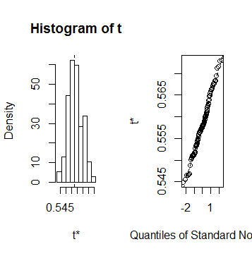
The value of the R-squared was about 0.55797 in every samples, no big differences occured.
Forward method
The Forward method begins with an empty model. First it selects the independent variable, in which case the absolute value of the correlation between this variable and the dependent variable is the maximum. Second it selects one with the largest partial correlation, i.e. the one with the maximal correlation after the first selected variable. Hereinafter entering variables it also takes account of the partial correlations, which is among the entering independent and the dependent variable, taking into account the other entered variables. The order of the explanatory variables matters (the later entrants are less and less able to increase the explanatory power of the model, matter what variables are already in). The entered variables are staying in the model.
> forward_actual_results<-rep(0,6)
> names(forward_actual_results)<-c("r_square","A","B","C","D","E")
>
> selection_forward<-function(data,num)
+ {
+   data<-data[num,]
+   fit <- forward(lm(X ~ A + B + C + D + E, data))
+
+   forward_actual_results[1]<-as.numeric(summary(fit)$r.square)
+
+   actual_selected<-rownames(summary(fit)$coef)[-1]
+   forward_actual_results[which(names(forward_actual_results) %in% actual_selected)]<-
+     forward_actual_results[which(names(forward_actual_results) %in% actual_selected)]+1
+   return(forward_actual_results)
+ }
>
> forward_results<-boot(data=data, statistic=selection_forward,
+                        R=100)
> forward<-summary(forward_results)
> rownames(forward)<-c("R-squared", "A", "B", "C", "D", "E")
> forward
            R original  bootBias   bootSE bootMed
R-squared 100  0.55754 -0.017099 0.040908 0.55754
A         100  1.00000  0.000000 0.000000 1.00000
B         100  1.00000  0.000000 0.000000 1.00000
C         100  1.00000 -0.150000 0.358870 1.00000
D         100  0.00000  0.200000 0.402015 0.00000
E         100  1.00000 -0.150000 0.358870 1.00000
The explanatory power of the model is the same as by the enter method, the value of R-squared was about 0.55754. In most of the models the D variable was left out, in some cases the C and E variables to. The A and B variables were always in.
Backward elimination
The Backward elimination, as the name suggests, essentially works in reverse as the Forward Method: in the beginning all independent variables are in the model, and the algorithm excludes those, which don’t significantly reduce the model’s explanatory power.
> backward_actual_results<-rep(0,6)
> names(backward_actual_results)<-c("r_square","A","B","C","D","E")
>
> selection_backward<-function(data,num)
+ {
+   data<-data[num,]
+   fit <- backward(lm(X ~ A + B + C + D + E, data))
+
+   backward_actual_results[1]<-as.numeric(summary(fit)$r.square)
+
+   actual_selected<-rownames(summary(fit)$coef)[-1]
+   backward_actual_results[which(names(backward_actual_results) %in% actual_selected)]<-
+     backward_actual_results[which(names(backward_actual_results) %in% actual_selected)]+1
+   return(backward_actual_results)
+ }
>
> backward_results<-boot(data=data, statistic=selection_backward,
+                         R=100)
> backward<-summary(backward_results)
> rownames(backward)<-c("R-squared", "A", "B", "C", "D", "E")
> backward
            R original   bootBias    bootSE bootMed
R-squared 100  0.55754 -0.0001725 0.0033409 0.55754
A         100  1.00000  0.0000000 0.0000000 1.00000
B         100  1.00000  0.0000000 0.0000000 1.00000
C         100  1.00000  0.0000000 0.0000000 1.00000
D         100  0.00000  0.2400000 0.4292347 0.00000
E         100  1.00000  0.0000000 0.0000000 1.00000
The results by the Backward elimination were more stable, while the value of the R-squared was the same as by the forward method. The A, B, C and E variableswere always included, the variable D was mostly excluded.
Stepwise selection
The Stepwise method is similar to the Forward method, in a sense it is its “improved” version: first enters the variable with the largest absolute value of the correlation and passing in the same way further than the Forward Method. Always enters the variable with the largest absolute value of partial correlation. However, the model continues to step backwards to check, and if there is a variable, that would not significantly reduce the explanatory power of the model when excluded, it drops out. New variables may change the partial correlation of the variables inside, “can reduce their attractiveness”. We can say stepwise selection is “better” than forward and backward methods in the way that it takes into account the predicting variables together, but we can not trust it blindly and we have to check if the model makes sense. An often mentioned example is that people look good from the outside in jeans and T-shirt but we know it is better if we wear underwear as well even if it is less effective and time consumming to put it on.
> stepWise_actual_results<-rep(0,6)
> names(stepWise_actual_results)<-c("r_square","A","B","C","D","E")
>
> selection_stepWise<-function(data,num)
+ {
+   data<-data[num,]
+   fit <- stepWise(lm(X ~ A + B + C + D + E, data))
+
+   stepWise_actual_results[1]<-as.numeric(summary(fit)$r.square)
+
+   actual_selected<-rownames(summary(fit)$coef)[-1]
+   stepWise_actual_results[which(names(stepWise_actual_results) %in% actual_selected)]<-
+     stepWise_actual_results[which(names(stepWise_actual_results) %in% actual_selected)]+1
+   return(stepWise_actual_results)
+ }
>
> stepWise_results<-boot(data=data, statistic=selection_stepWise,
+                        R=100)
> stepWise<-summary(stepWise_results)
> rownames(stepWise)<-c("R-squared", "A", "B", "C", "D", "E")
> stepWise
            R original  bootBias   bootSE bootMed
R-squared 100  0.55754 -0.030778 0.050863 0.55754
A         100  1.00000  0.000000 0.000000 1.00000
B         100  1.00000  0.000000 0.000000 1.00000
C         100  1.00000 -0.270000 0.446196 1.00000
D         100  0.00000  0.000000 0.000000 0.00000
E         100  1.00000 -0.270000 0.446196 1.00000
The value of the R-squared was the same as by the Forward and Backward methods. The variables A and B were always in, the D was aways out and the C and E were mostly included.
